|
Network Integration
Table of Contents
1. Introduction
The Network Integration module enables you to visualize and analyze multi-omics data in the context of biological networks. Rather than treating features as isolated entities, network integration provides biological context by mapping features onto molecular interaction networks, regulatory networks, and metabolic pathways.
- Provides biological context for statistical findings
- Identifies functional modules and network communities
- Discovers hub features with potential regulatory roles
- Enables interpretation of coordinated changes across omics layers
- Generates testable mechanistic hypotheses
The Network Integration workflow consists of three main steps:
- Database Selection - Choose from protein-protein interaction, metabolic, regulatory, and other network databases
- Network Builder - Construct multi-omics networks connecting genes, proteins, metabolites, and microbiome
- Network Viewer - Interactive visualization with functional enrichment analysis
2. Two Entry Points to Network Integration
There are two ways to access Network Integration, depending on your workflow:
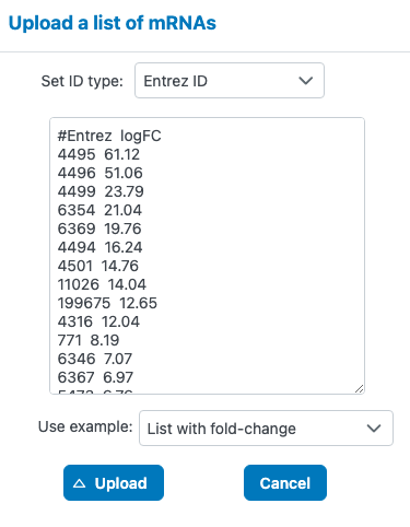
Entry Point 1: Upload Mode 2 (Feature Lists)
Directly upload pre-identified feature lists from external analysis tools (limma, DESeq2, edgeR, etc.) for network-based analysis.
- Upload one or more feature lists (genes, proteins, metabolites, etc.)
- Specify the model organism (Human, Mouse, or Other)
- For microbiome data, specify its host organism
Feature List Format
- First column: Feature identifiers (gene symbols, protein IDs, metabolite names, etc.)
- Second column (optional): Statistical values such as fold change, log2FC, or other numerical measures
- How these genes connect through known protein-protein interactions
- Which pathways are enriched among your gene list
- Hub genes that may play central regulatory roles
- Nodes colored by fold change to visualize expression patterns in network context
Entry Point 2: From Statistical Integration ("Functional exploration")
When you have completed statistical analysis using Upload Mode 1 (Data Tables), you can directly send significant features to Network Integration using the "Functional exploration" button. See the Statistical Integration Tutorial - Next Steps for detailed instructions.
- Available from limma results, variance decomposition, and other statistical analyses
- Automatically transfers significant features with their statistical values
- No need to export and re-upload feature lists
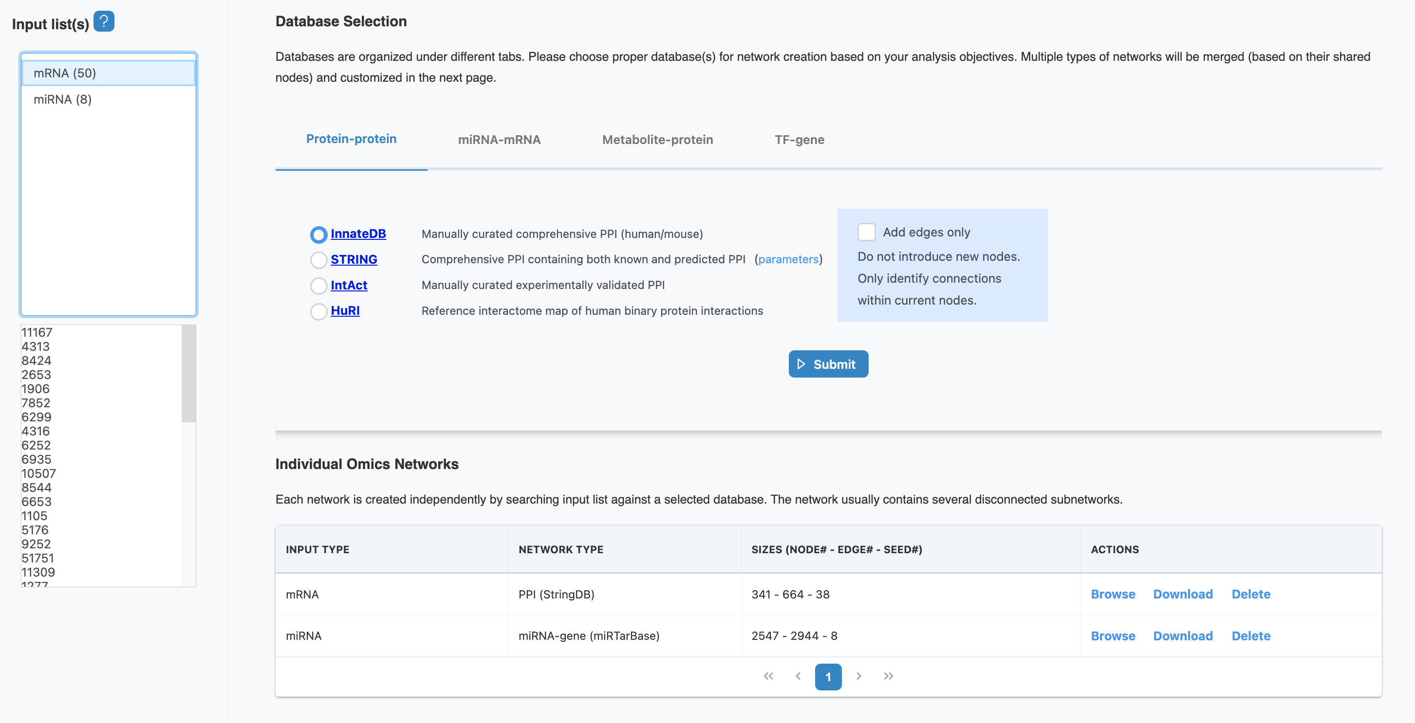
3. Database Selection
OmicsAnalyst 2.0 provides access to multiple curated molecular network databases. Choose the appropriate databases based on your omics types and research questions.
Available Network Databases
Protein-Protein Interaction (PPI)
Physical and functional protein interactions from STRING, BioGRID, and IntAct databases. Ideal for proteomics and transcriptomics data.
Metabolic Networks
Enzyme-metabolite relationships from KEGG, Reactome, and HumanCyc pathway databases. Essential for metabolomics integration.
Gene Regulatory Networks
Transcription factor-target gene relationships from ENCODE, ChIP-Atlas, and RegNetwork. Use for transcriptomics and epigenomics.
miRNA Regulatory Networks
miRNA-target gene interactions from miRTarBase, TargetScan, and miRDB. For small RNA and transcriptomics integration.
Signaling Networks
Signaling pathways and cascades from KEGG, Reactome, and WikiPathways. Captures dynamic cellular response pathways.
Microbiome Networks
Host-microbiome interactions connecting microbial taxa with host genes, proteins, and metabolites.
Database Selection Parameters
| Parameter | Description | Recommendation |
|---|---|---|
| Organism | Species for network database queries | Select your study organism (human, mouse, etc.) |
| Confidence Score | Minimum confidence threshold for interactions | 0.4-0.7 (medium to high confidence) |
| Evidence Types | Types of supporting evidence for interactions | Experimental, database, text-mining |
4. Network Builder
The Network Builder constructs multi-omics networks by mapping your input features onto the selected databases and extracting relevant interactions. If more than one network was generated, they will be merged together through shared nodes.
Network Overview
The network overview table displays all generated subnetworks with key statistics:
- Seed nodes: Your input query features that were mapped to the database
- All nodes: Total nodes including seeds and connecting nodes from the database
- Edges: Number of interactions/relationships in the network
- Topology: View network topology statistics (diameter, radius, clustering coefficient)
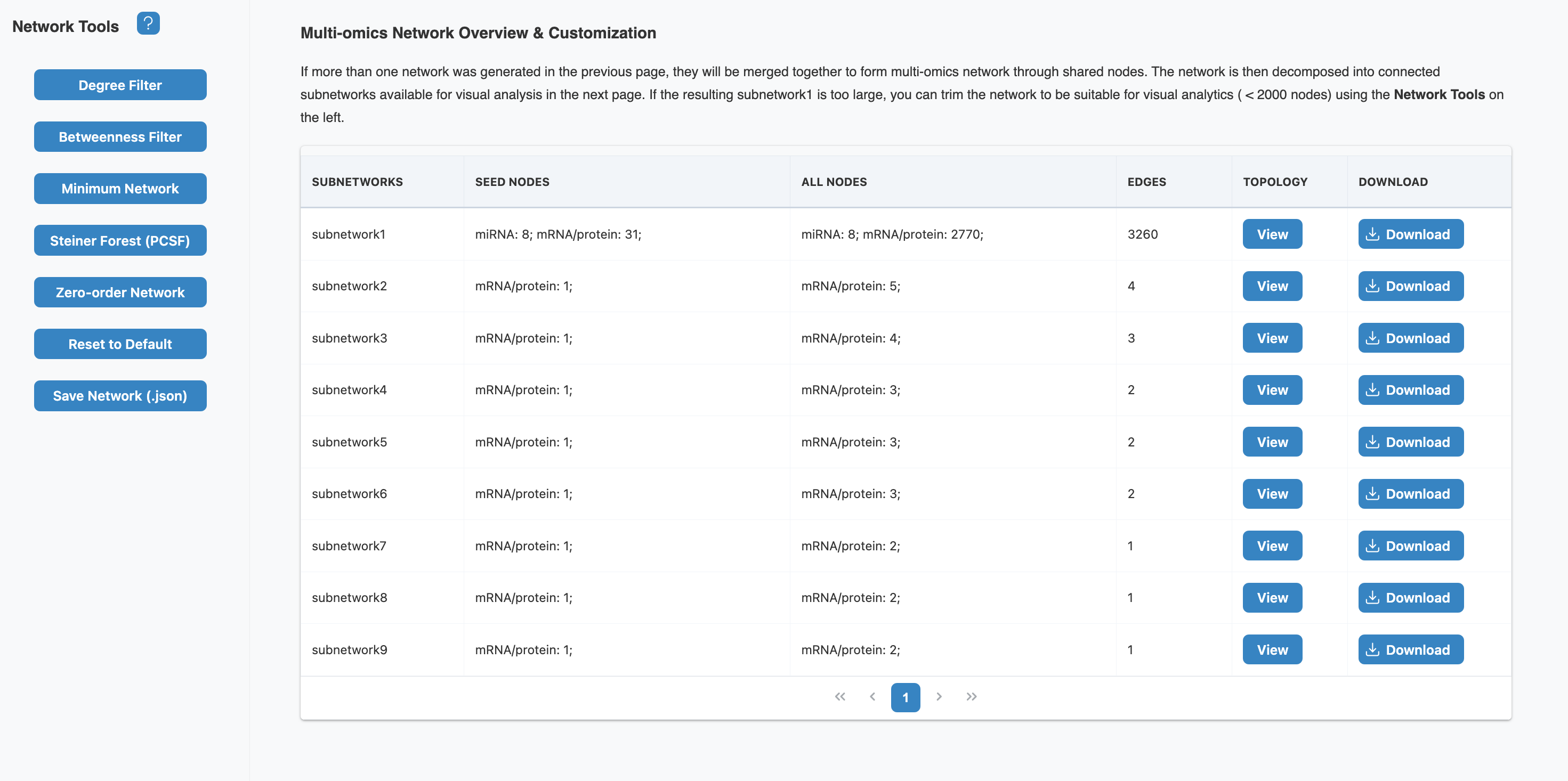
Network Tools
Large and dense networks can be difficult to navigate or interpret. Use the Network Tools to simplify the network while preserving key biological information:
Filtering Tools
- Degree Filter: Keep nodes with high connectivity (hubs). Nodes with higher degree act as important network hubs.
- Betweenness Filter: Keep nodes that bridge different modules. Nodes with higher betweenness act as important bottlenecks.
Network Reduction Tools
- Minimum Network: Keep seeds and essential non-seed nodes that maintain network connectivity. Based on Steiner Tree approximation - suitable for simplifying dense networks.
- Steiner Forest (PCSF): Identify context-specific subnetworks enriched with input queries from the global interaction network.
- Zero-order Network: Show only direct interactions between your query nodes (seeds), removing all intermediate nodes.
Other Tools
- Reset to Default: Restore the network to its original state
- Save Network (.json): Export the network in JSON format for external use
5. Network Viewer
The Network Viewer provides interactive visualization and exploration tools to analyze your multi-omics network.
Visualization Features
| Feature | Description |
|---|---|
| Layout Algorithms | Force-directed, hierarchical, circular, and grid layouts for optimal network visualization |
| Node Coloring | Map node colors to omics data (fold change, p-value) or network properties (degree, module) |
| Node Sizing | Scale node size by degree, betweenness centrality, or expression level |
| Edge Styling | Differentiate edge types (PPI, regulatory, metabolic) by color and style |
| Module Highlighting | Highlight detected network communities and functional modules |
Network Analysis Tools
Topology Metrics
Calculate and visualize network topology to identify key features:
- Degree: Number of connections (high-degree nodes are potential hubs)
- Betweenness: Frequency on shortest paths (bridging nodes between modules)
- Clustering Coefficient: Local connectivity (nodes in dense functional modules)
- Eigenvector Centrality: Influence based on connections to important nodes
Community Detection
Identify densely connected modules within the network. These modules often correspond to functional units such as pathways, protein complexes, or co-regulated gene sets.
- Louvain: Fast, multi-resolution community detection
- Walktrap: Random walk-based module detection
- Edge Betweenness: Hierarchical community structure
Interactive Exploration
- Navigate Network: Pan, zoom, and rotate to explore different regions of the network.
- Select Nodes: Click nodes to view detailed information including omics data and annotations.
- Highlight Paths: Select two nodes to highlight shortest paths between them.
- Filter Display: Toggle visibility of node types, edge types, or modules.
- Export: Save high-resolution images (PNG, SVG) and network data (JSON, GraphML) for publication.
6. Functional Enrichment
Perform pathway and functional enrichment analysis on your network to understand the biological processes represented by your multi-omics findings.
Enrichment analysis tests whether your network features are overrepresented in specific biological pathways (KEGG, Reactome) or functional categories (GO terms). You can perform enrichment on the entire network or on specific modules to understand their distinct biological functions.
Enrichment Workflow
- Select Features: Choose entire network, specific modules, or high-centrality nodes for enrichment analysis.
- Choose Databases: Select pathway/GO databases relevant to your organism and research question.
- Run Analysis: Execute enrichment with appropriate background gene set and multiple testing correction.
- Visualize Results: Explore bar charts, bubble plots, and enrichment maps of significant terms.
- Interpret Findings: Connect enriched pathways to your biological hypothesis and experimental design.
- Background: Use whole genome or expressed genes as background for accurate statistics
- P-value correction: FDR (Benjamini-Hochberg) or Bonferroni for multiple testing
- Minimum gene set size: Filter out very small pathways (typically min 10 genes)
- Maximum gene set size: Filter out very broad pathways (typically max 500 genes)
7. Interpreting Your Results
Let's walk through an example interpretation using the built-in "Two Lists" example dataset, which contains gene and miRNA lists from a brain cancer study (50 genes + 30 miRNAs).
Example: Gene-miRNA Regulatory Network from Brain Cancer Study
This example uses the "Two Lists" sample data available when you click "Try Example" on the upload page. The 50 genes (Entrez IDs) were queried against STRING (PPI database) and the 30 miRNAs against miRTarBase (miRNA-target database).
Step 1: Understanding Network Construction
Two separate networks were generated from different databases:
- Gene → PPI Network (STRING): 50 input genes mapped to 341 total nodes connected by 664 protein-protein interactions (38 seeds successfully mapped)
- miRNA → Target Network (miRTarBase): 30 input miRNAs expanded to 2,547 nodes (miRNAs + their validated target genes) with 2,944 regulatory edges (8 seeds with known targets)
These networks are then merged through shared gene nodes, creating an integrated gene-miRNA regulatory network.
Step 2: Network Merging and Subnetwork Detection
The Network Builder shows 9 subnetworks after merging:
- Subnetwork1 (main): Contains 8 mRNA seeds + 31 miRNA-related nodes → expanded to 2,770 nodes with 3,260 edges. This is the primary connected component where most biological signal resides.
- Subnetwork2-9: Smaller disconnected components (1-5 seeds each) representing features without known connections to the main network in current databases.
Interpretation: Most input features (39 of 58 seeds) participate in an interconnected regulatory network, suggesting coordinated biological function.
Step 3: Network Simplification with Minimum Network
The original Subnetwork1 (2,770 nodes) is too large for effective visualization. We applied the Minimum Network tool to extract only the essential structure connecting our seed nodes.
- What it does: Keeps all seed nodes plus the minimum set of connector nodes needed to maintain network connectivity (based on Steiner Tree approximation)
- Result: A simplified network that preserves the key biological relationships while removing peripheral nodes
- When to use: When your network exceeds ~500 nodes and becomes difficult to interpret visually
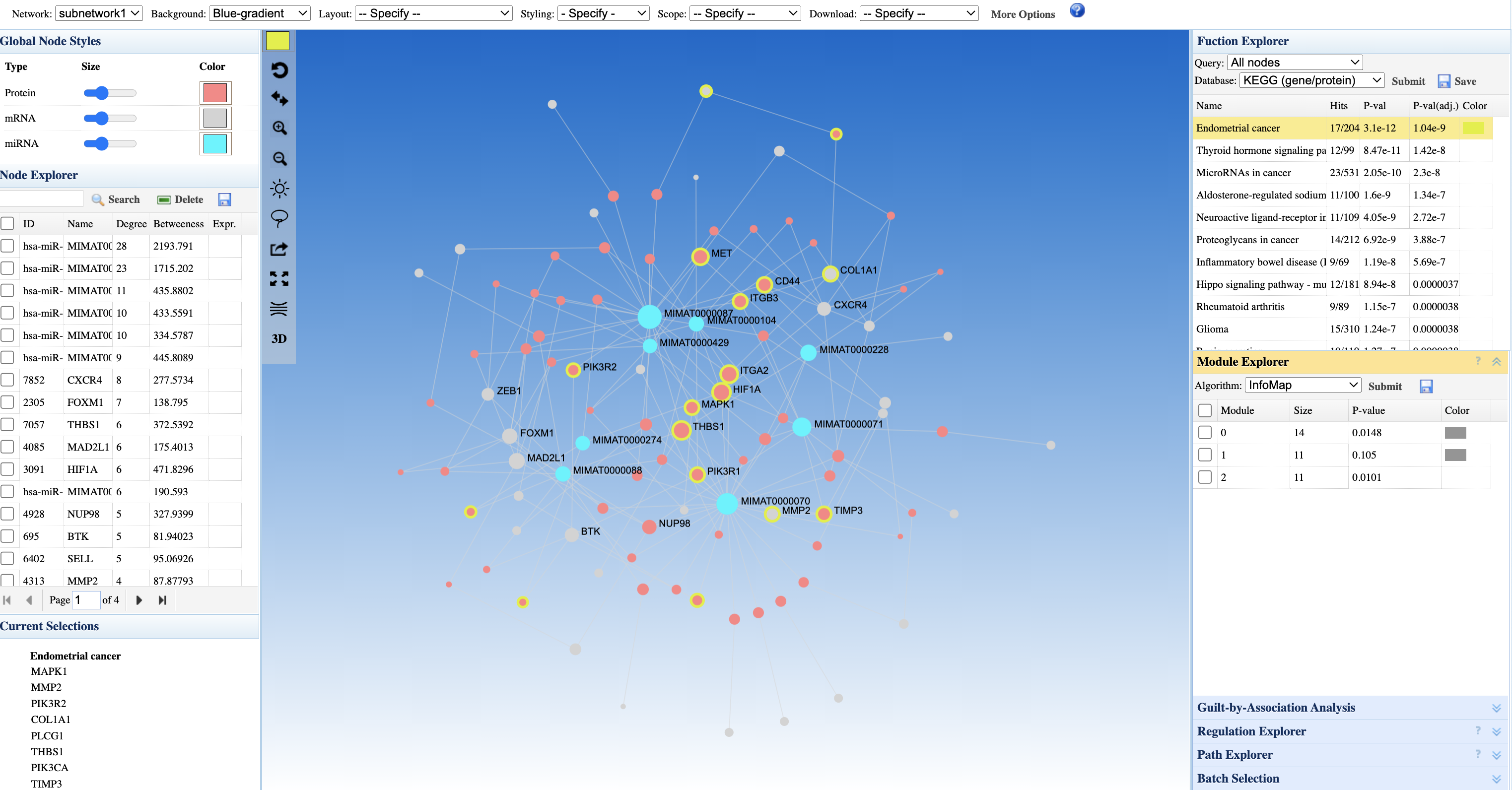
Step 4: Understanding the Network Visualization
The Network Viewer displays the simplified minimum network with multiple visual encodings:
- Node colors (Blue-gradient): Intensity reflects the statistical value (e.g., fold change) from your input - darker colors indicate stronger differential expression
- Node types: Different node styles distinguish mRNAs/proteins from miRNAs (see Global Node Styles legend)
- Orange/yellow highlighted nodes: Your seed features are emphasized (e.g., labeled nodes like MMATR0000074)
- Connector nodes: Non-seed nodes retained by the Minimum Network algorithm - these are essential bridges connecting your seeds
- Edge types: PPI edges (protein-protein) vs. regulatory edges (miRNA-target) may be styled differently
Step 5: Interpreting Pathway Enrichment
The Function Explorer panel shows KEGG pathway enrichment results:
- Endometrial cancer (17/54 genes, p = 1.4e-6): The top enriched pathway - 17 genes from your network overlap with this cancer pathway
- Thyroid hormone signaling pathway (p = 8.3e-5): Suggests involvement in hormone-responsive signaling
- MicroRNAs in cancer (p = 4.8e-6): Confirms the cancer-regulatory role of your miRNA seeds
- Hippo signaling pathway, Glioma: Additional cancer-related pathways
Biological interpretation: The convergence on cancer pathways (especially endometrial cancer) suggests your differentially expressed mRNAs and miRNAs may be involved in oncogenic processes. The miRNAs likely regulate genes within these cancer pathways.
Step 6: Exploring Network Topology
The Node Explorer table ranks features by network centrality:
- Degree (connectivity): High-degree nodes (e.g., hsa-miR-MIRNA74-13 with degree 1,713) are highly connected hubs - these miRNAs regulate many target genes
- Betweenness (bridging): High-betweenness nodes connect different network regions - these may be key regulatory bottlenecks
- Seed status: Your input features are marked, allowing you to distinguish seeds from database-added connector nodes
Step 7: Module-Specific Analysis
The Module Explorer identifies functional communities within the network:
- Module 0, 1, 2, 3: Four detected modules with varying sizes and p-values
- Each module represents a densely connected subgroup that may correspond to a distinct biological process
- Run enrichment on individual modules to understand their specific functions
- Regulatory mechanism: The miRNAs from the brain cancer study target genes that interact with the 50 differentially expressed genes through protein-protein interactions
- Pathway context: These genes converge on cancer-related pathways, suggesting involvement in oncogenic processes
- Key regulators: Hub miRNAs with high degree may be master regulators worth prioritizing for experimental validation
- Testable hypothesis: The identified miRNAs may suppress or activate cancer pathways by targeting key genes - this can be validated through functional experiments
8. Next Steps
After building and analyzing your network, you can proceed with causal analysis to test mechanistic hypotheses.
If you uploaded feature lists directly (Entry Point 1), you will need to return to Upload Mode 1 with your data tables to access Causal Analysis.
- Test whether a hub transcription factor mediates the relationship between upstream regulators and downstream targets
- Identify interaction effects between metabolites and genes in connected network modules
- Validate putative regulatory relationships discovered through network topology
Continue to the Causal Analysis Tutorial to learn about mediation analysis and interaction modeling (IntLIM).
